Butterflies and Roses With Julia

I recently came across this tumblr post by Mathhombre in which he had shared some beautiful plots he generated using Geogebra. Since it has been so long since I’ve tried anything with Julia, I thought of recreating some of those plots using Julia. Hence, this post.

In order to plot, make sure you have the following libraries installed.

1
2
3
using Plots
using PlutoUI
using ColorSchemes

Butterflies

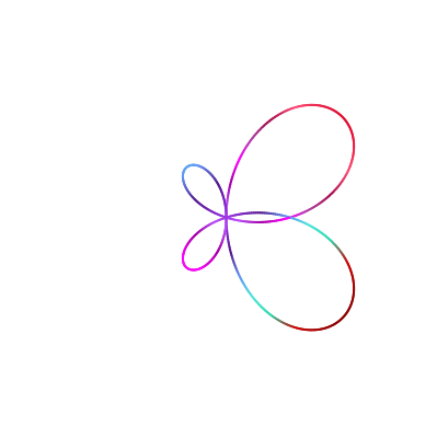
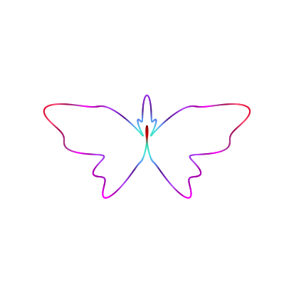
These plots are originally attributed to Daniel Mentrard. He has a large collections of math geogebra projects. One of them is to plot butterflies using polar curves. It is an easy task to reproduce them in Julia. Refer to the $r(\theta)$ formula in the Julia code to find the corresponding equation for each of these plots.

Buttefly #1

1
2
3
4
5
6
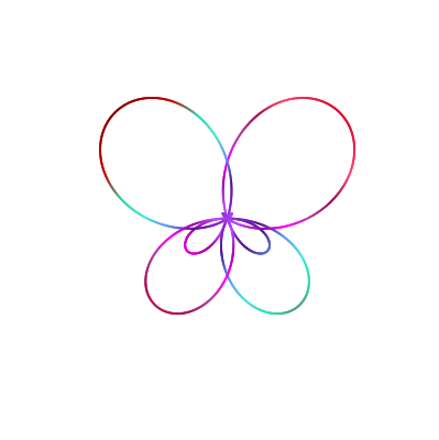
r(θ) = 5sin(2θ) + 3cos(θ)
rval = r.(0:0.01:2π)
p = plot(r, 0:0.01:2π, 
    proj=:polar, legend=false, linewidth=2, grid=:none, showaxis=false,
    linez=rval, c=:dracula, 
    background_color = :transparent, size=(400,400))

Butterfly 1

Butterfly #2

 1
 2
 3
 4
 5
 6
 7
 8
 9
10
11
12
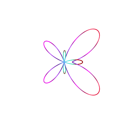
r1(θ) = (sin(5θ) + 3cos(θ))
r2(θ) = (sin(5θ) - 3cos(θ))
r1val = r1.(0:0.01:2π)
r2val = r2.(0:0.01:2π)
p = plot(r1, 0:0.01:2π, proj=:polar, legend=false, linewidth=2,
        grid=:none, showaxis=false,
        linez=r1val, c=:dracula,
        background_color = :transparent, size=(400,400));
plot!(p, r2, 0:0.01:2π, proj=:polar, legend=false, linewidth=2,
    grid=:none, showaxis=false,
    linez=r2val, c=:dracula,
    background_color = :transparent, size=(400,400))

Butterfly #3

 1
 2
 3
 4
 5
 6
 7
 8
 9
10
11
12
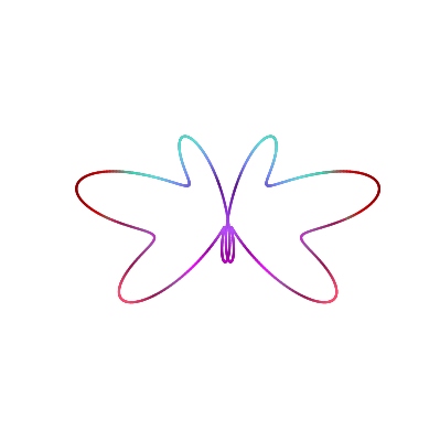
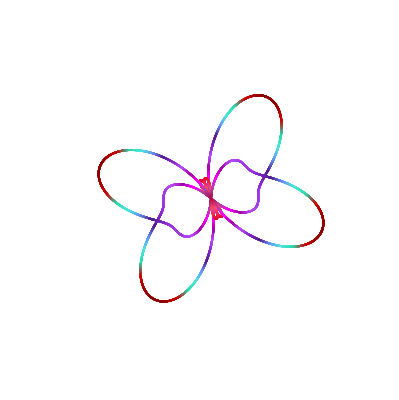
r1(θ) = 3cos(θ) + sin(7θ)
r2(θ) = -3cos(θ) + sin(7θ)
r1val = r1.(0:0.01:2π)
r2val = r2.(0:0.01:2π)
p = plot(r1, 0:0.01:2π, proj=:polar, legend=false, linewidth=2,
        grid=:none, showaxis=false,
        linez=r1val, c=:dracula,
background_color = :transparent, size=(400,400));
plot!(p, r2, 0:0.01:2π, proj=:polar, legend=false, linewidth=2,
    grid=:none, showaxis=false,
    linez=r2val, c=:dracula,
background_color = :transparent, size=(400,400))

Butterfly #4

1
2
3
4
5
6
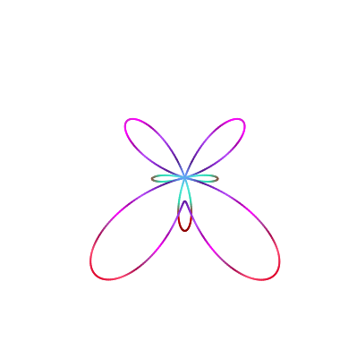
r(θ) = 2sin(2θ)+2cos(0.5θ)
rval = r.(0:0.01:4π)
p = plot(r, 0:0.01:4π, 
    proj=:polar, legend=false, linewidth=2, grid=:none, showaxis=false,
    linez=rval, c=:dracula,
    background_color = :transparent, size=(400,400))

Butterfly #5

1
2
3
4
5
6
r(θ) = exp(-sin(θ)) - 2cos(4θ) + (sin((2θ-π)/24)^4)
rval = r.(0:0.01:2π)
plot(r, 0:0.01:2π, 
    proj=:polar, legend=false, linewidth=2, grid=:none, showaxis=false,
    linez=rval, c=:dracula,
    background_color = :transparent, size=(400,400))

Butterfly #6

1
2
3
4
5
6
r(θ) = 1.6 + 1.1cos(2θ) + (sin(5θ)^3)
rval = r.(0:0.01:2π)
plot(r, 0:0.01:2π, 
    proj=:polar, legend=false, linewidth=2, grid=:none, showaxis=false,
    linez=rval, c=:dracula,
    background_color = :transparent, size=(400,400))

Butterfly #7

1
2
3
4
5
6
r(θ) = exp(sin(θ)-2cos(4θ))
rval = r.(0:0.01:2π)
plot(r, 0:0.01:2π, 
    proj=:polar, legend=false, linewidth=2, grid=:none, showaxis=false,
    linez=rval, c=:dracula,
background_color = :transparent, size=(400,400))

Butterfly #8

1
2
3
4
5
6
r(θ) = exp(cos(θ)) - 2cos(4θ) + (sin(θ/12)^7)
rval = r.(0:0.01:2π)
plot(r, 0:0.01:2π, 
    proj=:polar, legend=false, linewidth=2, grid=:none, showaxis=false,
    linez=rval, c=:dracula,
    background_color = :transparent, size=(400,400))

Butterfly #9

 1
 2
 3
 4
 5
 6
 7
 8
 9
10
11
12
13
14
15
16
17
18
a = -2
b = 2
c = 1
d = 4
K = -2.8
r1(θ) = a*sin(b*θ) + c*sin(d*θ) + K
r2(θ) = a*cos(b*θ) + c*sin(d*θ) + K

r1val = r1.(0:0.01:20π)
r2val = r2.(0:0.01:20π)
p = plot(r1, 0:0.01:20π, proj=:polar, legend=false, linewidth=2,
        grid=:none, showaxis=false, lims=(-1,4),
        linez=r1val, c=:dracula,
        background_color = :transparent, size=(400,400));
plot!(p, r2, 0:0.01:20π, proj=:polar, legend=false, linewidth=2,
    grid=:none, showaxis=false, lims=(-1,4),
    linez=r2val, c=:dracula,aspectratio=:equal,
    background_color = :transparent, size=(400,400))

Roses

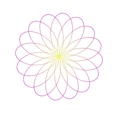
While plotting the buttefly wasn’t difficult, plotting the roses are even easier, thanks to Pluto.jl’s support for HTML slider objects being binded to variable. Hence, the equations,

$$ r_1(\theta) = a\sin(b\theta) + csin(d\theta) + K $$ $$ r_2(\theta) = a\cos(b\theta) + csin(d\theta) + K $$

with parameters $a,b,c,d,K$ were easier to set. Here are some beautiful flowers rendered with Julia and gr plot backend.

Rose #1

1
2
3
4
5
6
7
8
r(θ) = 4sin(-3.2θ) + 3.9
rval = r.(0:0.01:10π)
plot(r, 0:0.01:10π, proj= :polar, legend=false,linewidth=1, 
    mode="lines", axis=false, grid=:none, 
    aspectratio=:equal, lims=:auto,
    linez=rval,
    c=cgrad(:buda,rev=true),
    background_color = :transparent, size=(400,400))

Rose #2

1
2
3
4
5
6
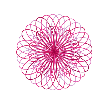
r(θ) = 3.3sin(3.3θ) + 0.6
rval = r.(0:0.01:30π)
plot(r, 0:0.01:30π, 
    proj=:polar, legend=false, linewidth=2, grid=:none, showaxis=false, 
    linez=range(minimum(rval),stop=maximum(rval),length=length(rval)), c=:PuRd_8,
    background_color = :transparent, size=(400,400))

Rose #3

 1
 2
 3
 4
 5
 6
 7
 8
 9
10
11
12
13
14
15
16
17
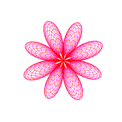
a = -2
b = 2.9
c = 3
d = 4
K = 0
r1(θ) = a*sin(b*θ) + c*sin(d*θ) + K
r2(θ) = a*cos(b*θ) + c*sin(d*θ) + K
r1val = r1.(0:0.01:20π)
r2val = r2.(0:0.01:20π)
p = plot(r1, 0:0.01:20π, proj=:polar, legend=false, linewidth=1,
        grid=:none, showaxis=false,
        c=:spring,aspectratio=:equal,
        background_color = :transparent, size=(400,400));
plot!(p, r2, 0:0.01:20π, proj=:polar, legend=false, linewidth=1,
    grid=:none, showaxis=false,
    c=:red,aspectratio=:equal,
    background_color = :transparent, size=(400,400))

Rose #4

 1
 2
 3
 4
 5
 6
 7
 8
 9
10
11
12
13
14
15
16
17
18
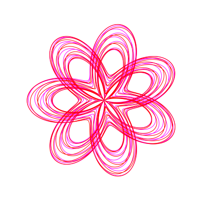
a = -1
b = 0.777
c = 2
d = 3.5
K = 3.
r1(θ) = a*sin(b*θ) + c*sin(d*θ) + K
r2(θ) = a*cos(b*θ) + c*sin(d*θ) + K
theta = 0:0.01:33π
r1val = r1.(theta)
r2val = r2.(theta)
p = plot(r1, theta, proj=:polar, legend=false, linewidth=1,
        grid=:none, showaxis=false,
        c=:spring,aspectratio=:equal,
        background_color = :transparent, size=(400,400));
plot!(p, r2, theta, proj=:polar, legend=false, linewidth=1,
    grid=:none, showaxis=false,
    c=:red,aspectratio=:equal,
    background_color = :transparent, size=(400,400))

Rose #∞

Pluto notebook of Julia supports html sliders to be bound to variable values. This allows us to use the sliders and generate the required plots.

1
@bind a Slider(-4:0.1:4, default=-2, show_value=true)

The pluto notebook is uploaded to Github gist can be accessed with Binder using this link. Further, the Pluto notebook can be downloaded from the following Github gist.