In this post, we will look at a way of approximating deflection function of beams using Rayleigh Ritz method. I had been recently watching this (click here for youtube link) lecture series by Clayton Pettit which had been a very useful introduction to finite element methods. This is one of the assignment problems provided in that series.
Regarding the choice of language here, it is Julia but also python (through PyCall, but for sympy that’s taken care by the SymPy package). The reason for this acrobatics is that python had issues converting singularity functions which tend to rise when analytically solving the system using Singularity method (if that sounds like gibberish, I would suggest “Machine Design, an Integrated Approach by Norton” for a quick brush up). I did initially intend to use Julia but the symbolics library doesn’t have all the calculus functionalities yet. Now, let’s get started!
| |
| |
Problem Statement
Consider the following cantilever beam.
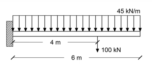
The value for various parameters in the problem are defined as following:
| |
0.0031249999999999997
Consider an Euler-Bernoulli beam (with the assumptions). The deflection of the beam can be obtained by solving the loading equation,
$$\displaystyle{q= EI\left( \frac{d^2y}{dx_1^2} \right) }$$
with the boundary conditions,
$$y(x_1=0) = 0$$ $$\frac{dy}{dx}(x_1=0) = 0$$
Further, there are the implicit boundary conditions, $\displaystyle{V(0^-)=0, M(0^-)=0, V(l^+)=0, M(l^+)=0 }$ which are utilised to solve the equation analytically.
If the above equation is solved, the shear force $V$ and bending moment $M$ can be obtained through, $$\displaystyle{M = EI\left( \frac{d ^2y}{d x_1^2} \right) }$$ $$\displaystyle{V = EI\left( \frac{d ^3y}{d x_1^3} \right) }$$
Rayleigh Ritz Method
Solving the above equation becomes tedious as the complexity of the loading increases. Hence, one might often resort to approximations. Rayleigh-Ritz method is one such method of approximating the deflection equation. This can be broken down into the following steps.
- Approximate the function to be solved for as a polynomial
- Apply boundary conditions
- Find the potential energy with this equation and minimize it by taking variations with respect to the parameters.
- Solve the arising equations to find the constants. Substitute them back to get the approximate function.
Approximation function
Let’s start with the approximation of the deflection as a polynomial. Note that, the loading equation is a 4th order equation which means that our polynomial should have a minimum degree of 4. Here, we will take a polynomial of order 6 and see how it turns out.
| |
$a_{0} + a_{1} x_{1} + a_{2} x_{1}^{2} + a_{3} x_{1}^{3} + a_{4} x_{1}^{4} + a_{5} x_{1}^{5} + a_{6} x_{1}^{6}$
Boundary Conditions
The next step is to apply the boundary conditions on the $y_\text{approx}$. This is done below and the following values for the first two coefficients are obtained.
| |
(a0, a1)
| |
Dict{Any, Any} with 2 entries:
a1 => 0
a0 => 0
Substituting the boundary conditions, $y_\text{approx}$ is reduced to a polynomial with 5 coefficients.
| |
$a_{2} x_{1}^{2} + a_{3} x_{1}^{3} + a_{4} x_{1}^{4} + a_{5} x_{1}^{5} + a_{6} x_{1}^{6}$
Potential Energy
The next step is to find the potential energy which is given as,
In the above equation, the external work is given as,
$$\text{Work = W.D by UDL + W.D by Point Load + W.D by concentrated moments}$$
where, the concentrated moment doesn’t exist in our case. Hence, ignoring that, the rest is implemented as follows:
| |
$750000.0 a_{2}^{2} + 13500000.0 a_{2} a_{3} + 108000000.0 a_{2} a_{4} + 810000000.0 a_{2} a_{5} + 5832000000.0 a_{2} a_{6} + 81000000.0 a_{3}^{2} + 1458000000.0 a_{3} a_{4} + 11664000000.0 a_{3} a_{5} + 87480000000.0 a_{3} a_{6} + 6998400000.0 a_{4}^{2} + 116640000000.0 a_{4} a_{5} + 899794285714.286 a_{4} a_{6} + 499885714285.714 a_{5}^{2} + 7873200000000.0 a_{5} a_{6} + 31492800000000.0 a_{6}^{2}$
| |
$- 4840 a_{2} - 20980 a_{3} - 95584 a_{4} - 452320 a_{5} - \frac{15464320 a_{6}}{7}$
| |
$750000.0 a_{2}^{2} + 13500000.0 a_{2} a_{3} + 108000000.0 a_{2} a_{4} + 810000000.0 a_{2} a_{5} + 5832000000.0 a_{2} a_{6} + 4840 a_{2} + 81000000.0 a_{3}^{2} + 1458000000.0 a_{3} a_{4} + 11664000000.0 a_{3} a_{5} + 87480000000.0 a_{3} a_{6} + 20980 a_{3} + 6998400000.0 a_{4}^{2} + 116640000000.0 a_{4} a_{5} + 899794285714.286 a_{4} a_{6} + 95584 a_{4} + 499885714285.714 a_{5}^{2} + 7873200000000.0 a_{5} a_{6} + 452320 a_{5} + 31492800000000.0 a_{6}^{2} + \frac{15464320 a_{6}}{7}$
Finding Coefficients
Note that, $\prod(y(x_1))$ is a functional which means that it takes a function $y_{\text{approx}}(x_1)$ as input and gives a scalar as output. Our aim is to find the $y_{\text{approx}}$ which gives the minimum value of the potential energy. In order to find that, we differentiate $\prod$ with respect to each of the remaining coefficients ($\displaystyle{a_2, a_3, a_4, a_5, a_6}$). We solve the resulting system of equations algebraically to get the corresponding values. Note that, if we had not applied the boundary conditions initially, the coefficients $\displaystyle{a_0, a_1}$ can also be solved this way but that won’t gaurantee that the resulting equation will satisfy the boundary conditions.
| |
Dict{Any, Any} with 5 entries:
a6 => 1.42254737596294e-7
a3 => 0.000886803840876093
a4 => 8.40877915018096e-6
a2 => -0.00960098765431926
a5 => -5.12117055336974e-6
Approximate Solutions
Substituting these values back in the equation, we obtain the approximated equation for the deflection. Further, we substitute this equation in the equations for $M$ and $V$ to get the $\displaystyle{M_{\text{approx}}}$ and $\displaystyle{V_{\text{approx}}}$ respectively.
| |
$1.42254737596294 \cdot 10^{-7} x_{1}^{6} - 5.12117055336974 \cdot 10^{-6} x_{1}^{5} + 8.40877915018096 \cdot 10^{-6} x_{1}^{4} + 0.000886803840876093 x_{1}^{3} - 0.00960098765431926 x_{1}^{2}$
| |
$0.266727632993052 x_{1}^{4} - 6.40146319171217 x_{1}^{3} + 6.30658436263572 x_{1}^{2} + 332.551440328535 x_{1} - 1200.12345678991$
| |
$1.06691053197221 x_{1}^{3} - 19.2043895751365 x_{1}^{2} + 12.6131687252714 x_{1} + 332.551440328535$
Analytical Solution
In order to check the quality of approximation, we will compare it against the analytical solution which is given by, $$\displaystyle{y_{\text{act}}= \frac{1}{EI}\left( \frac{1}{2}M_1\left<x_1-0 \right>^2 + \frac{1}{6}R_1\left<x_1-0 \right>^3 + \frac{1}{24}qx_1^4 + \frac{1}{6}P\left<x_1-4 \right>^3 \right) }$$
where, $<\cdot>$ indicate the singularity functions, $R_1$ and $M_1$ are the reaction load and moment on the fixed end. The values are substituted and the $y_{\text{act}}$ is derived below.
The corresponding $M_{\text{act}}$ and $V_{\text{act}}$ are also calculated.
| |
$- 3.0 \cdot 10^{-5} x_{1}^{4} + 0.000986666666666667 x_{1}^{3} - 0.00968 x_{1}^{2} - 0.000266666666666667 {\left\langle x_{1} - 4 \right\rangle}^{3}$
| |
$- 22.5 x_{1}^{2} + 370.0 x_{1} - 100.0 {\left\langle x_{1} - 4 \right\rangle}^{1} - 1210.0$
| |
$- 45.0 x_{1} - 100.0 {\left\langle x_{1} - 4 \right\rangle}^{0} + 370.0$
Comparison
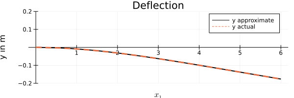
Deflection Plot
In the plot below, we are plotting the actual and approximated y values. It can be seen that approximation conforms very well to the original function.
| |
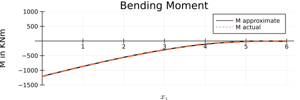
Bending Moment Diagram
In the bending diagram, the approximation still seems to hold good though there seems to be a something peculiar at $x_1=4$ but not enough to judge without careful examination.
| |
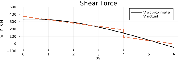
Shear Force Diagram
Now, while drawing the Shear force diagram, the caveats of approximation is seen. The area under the curve remains the same (aka the bending moment) but the actual curve traced is different. The analytical solution has the discontinuity at $x_1=4$ mark which is smoothed out. Also, the maximum shear force predicted is slightly lower than the analytical solution.
| |
Stress Calculations
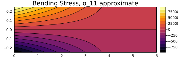
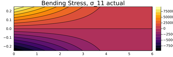
Next, we shall take a look at the bending and shear stresses. For an Euler-Bernoulli beam, only $\sigma_{11}$ and $\sigma_{12}$ exists which are given by,
$$\displaystyle{\sigma_{11} = \frac{Mx_2}{I}}$$
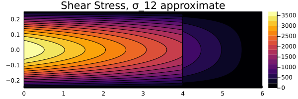
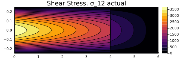
$$\displaystyle{\sigma_{12}= \frac{VQ}{Ib}}$$
where $\displaystyle{Q = b \left( \frac{t}{2}-x_2 \right) \left( \frac{t}{4}+\frac{x_2}{2} \right) }$ for a rectangular cross sectioned beam.
| |
$320.0 x_{2} \left(22.5 x_{1}^{2} - 370.0 x_{1} + 100.0 {\left\langle x_{1} - 4 \right\rangle}^{1} + 1210.0\right)$
| |
$320.0 x_{2} \left(- 0.266727632993052 x_{1}^{4} + 6.40146319171217 x_{1}^{3} - 6.30658436263572 x_{1}^{2} - 332.551440328535 x_{1} + 1200.12345678991\right)$
| |
$1066.66666666667 \left(0.075 - 0.3 x_{2}\right) \left(\frac{x_{2}}{2} + 0.125\right) \left(- 45.0 x_{1} - 100.0 {\left\langle x_{1} - 4 \right\rangle}^{0} + 370.0\right)$
| |
$1066.66666666667 \left(0.075 - 0.3 x_{2}\right) \left(\frac{x_{2}}{2} + 0.125\right) \left(1.06691053197221 x_{1}^{3} - 19.2043895751365 x_{1}^{2} + 12.6131687252714 x_{1} + 332.551440328535\right)$
In the following cells, the $\sigma_{11}$ and $\sigma_{12}$ actual and approximate values are plotted. Note that, if you run this in your system, the following plots may take a lot of time. This is due to sympy. A purely Julia based symbolic library would have meant lesser hassle.
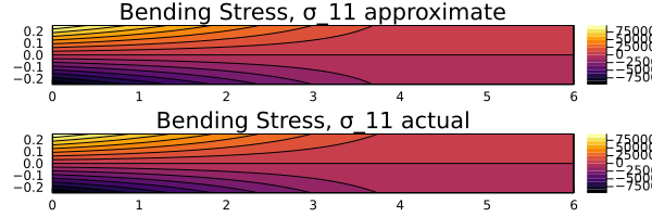
Bending Stress
| |
| |
| |
| |
Shear Stress
| |
Comparison
| |
| |
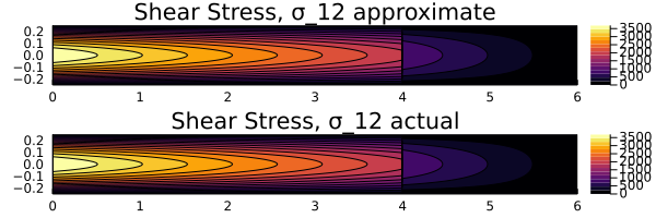
Based on the comparison above, it can be seen that the stress distributions for both $y_\text{act}$ and $y_\text{approx}$ remain the same. Hence, this can be considered as a viable approximation for the deflection function.
The entire blog post is a Jupter Notebook which can be downloaded from below. Please note that this is generated as a part of my learning experience and hence should be treated appropriately.