This post is meant as an introduction into a simple graphical optimization problem using Python. Consider a simply supported (Euler) beam of uniform rectangular cross section. The objective is to minimize the weight of the beam. Breadth (b) and depth (d) are variable. Length is fixed. Stresses must be within safe limits and mid deflection should be $\le$1% of the span.
1
2
3
4
5
| import numpy as np
import matplotlib as mpl
import matplotlib.pyplot as plt
from mpl_toolkits.mplot3d import proj3d
from matplotlib import patheffects
|
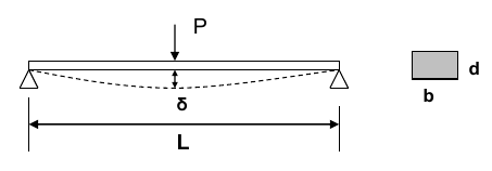
Here, the objective is to minimize $W = \rho b d L$ where b, d are the design variables. The constraints are,
- Mid span deflection ($\delta$) restricted to $L/100$ - $\frac{PL^3}{48EI} \le \frac L {100}$.
Substituting $I=\frac{bd^3}{12}$ we get, $\frac{PL^3}{4Ebd^3} \le \frac L {100}$.
- The maximum bending stress must not exceed yield stress ($\sigma_y$) - $\sigma = \frac{My}I \le \sigma_y$.
Substituting $M = \frac {PL}4$, $y=\frac d 2$ and $I=\frac{bd^3}{12}$, we get $\frac{3PL}{2bd^2} \le \sigma_y$.
In addition to these, since the beam is an Euler beam, a condition on slenderness must be implemented - say $d\le\frac L {10}$. Hence, the optimization problem can be formulated as follows:
$$
\begin{equation*}
\begin{aligned}
& \underset{b, d}{\text{minimize}}
& & W = \rho b d L \\
& \text{subject to}
& & \frac{PL^2}{4Ebd^3} - 0.01 \le 0 \\
& & & \frac {1.5PL}{bd^2} - \sigma_y \le 0 \\
& & & d - \frac L {10} \le 0
\end{aligned}
\end{equation*}
$$
Now, let’s substituted some numerical values. $L=1m$, $E=2\times 10^{11} N/m^2$, $\rho = 7000 kg/m^3$, $P=2000N$ and $\sigma_y = 200\text{MPa}$.
1
2
3
4
5
| L=1
E = 2e11
rho = 7000
P = 2000
sigma_y = 200e6
|
In addition to these, we will define the permissible range for the values of b and d, $0\le b \le 0.1$ and $0 \le d \le 0.1$.
1
2
| val_range = np.linspace(0.001, 0.1, 101)
b,d = np.meshgrid(val_range, val_range)
|
1
2
3
| g1 = (P*L**2/(4*E*b*d**3) - 0.01)
g2 = (1.5*P*L/(b*d**2)) - sigma_y
g3 = d - L/10
|
1
2
3
4
5
6
7
8
9
| fig = plt.figure(figsize=(10,10))
ax = plt.subplot(projection='3d')
ax.plot_surface(b, d, Obj, cmap="plasma", alpha=0.5)
ax.contour(b, d, Obj, zdir='z', offset=np.min(Obj), cmap="plasma", levels=25)
ax.set_title("Objective function")
ax.set_xlabel("b")
ax.set_ylabel("d")
ax.set_zlabel("W")
|
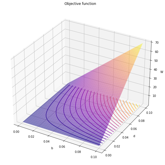
For the further analysis, we will make use of the contour plot (as show in the xy plane) to generate further graphics.
 1
 2
 3
 4
 5
 6
 7
 8
 9
10
11
12
13
14
15
16
17
18
| fig, ax = plt.subplots(figsize=(10,10))
obj_cntr = ax.contour(b, d, Obj, cmap="plasma", levels=25)
ax.clabel(obj_cntr, fmt="%2.1f", use_clabeltext=True)
cg1 = ax.contour(b, d, g1, [0], colors='sandybrown')
plt.setp(cg1.collections,
path_effects=[patheffects.withTickedStroke(angle=135)])
cg2 = ax.contour(b, d, g2, [0], colors='dodgerblue')
plt.setp(cg2.collections,
path_effects=[patheffects.withTickedStroke(angle=135)])
cg3 = ax.contour(b, d, g3, [0], colors='red')
plt.setp(cg3.collections,
path_effects=[patheffects.withTickedStroke(angle=-135)])
ax.annotate('Optima', xy=(0.0015,0.1), xytext=(0.01, .08), fontsize=16,
arrowprops=dict(facecolor='black', shrink=0.02),
)
ax.set_title("Contour plot")
ax.set_xlabel("b")
ax.set_ylabel("d")
|
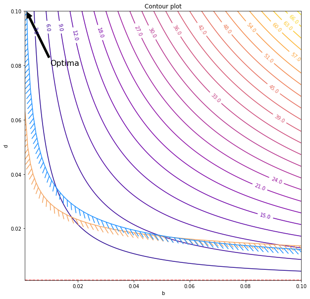
The minimum possible values are established by the maximum possible values for the two constraints which are represented by the stroked lines. Note that the third condition was satisfied by the entire domain in the plot. That means, we have a design space where the optima is achieved at,
$$b, d = (0.0015, 0.1)$$
However, this is a highly unrealistic ratio since $d/b = 66.67$. Hence we will impose another constraint as $b/d \ge 1/10$,
$$0.1 - \frac b d \le 0$$
 1
 2
 3
 4
 5
 6
 7
 8
 9
10
11
12
13
14
15
16
17
18
19
20
21
22
23
24
| g4 = 0.1 - b/d
d_optima = np.cbrt(15*P*L/(sigma_y))
b_optima = d_optima/10
fig, ax = plt.subplots(figsize=(10,10))
obj_cntr = ax.contour(b, d, Obj, cmap="plasma", levels=25)
ax.clabel(obj_cntr, fmt="%2.1f", use_clabeltext=True)
cg1 = ax.contour(b, d, g1, [0], colors='sandybrown')
plt.setp(cg1.collections,
path_effects=[patheffects.withTickedStroke(angle=135)])
cg2 = ax.contour(b, d, g2, [0], colors='dodgerblue')
plt.setp(cg2.collections,
path_effects=[patheffects.withTickedStroke(angle=135)])
cg3 = ax.contour(b, d, g3, [0], colors='red')
plt.setp(cg3.collections,
path_effects=[patheffects.withTickedStroke(angle=-135)])
cg4 = ax.contour(b, d, g4, [0], colors='red')
plt.setp(cg4.collections,
path_effects=[patheffects.withTickedStroke(angle=135)])
ax.annotate('Optima: (%.2f, %.2f)'% (b_optima, d_optima), xy=(b_optima, d_optima), xytext=(0.02, .04), fontsize=16,
arrowprops=dict(facecolor='black', shrink=0.02),
)
ax.set_title("Contour plot")
ax.set_xlabel("b")
ax.set_ylabel("d")
|
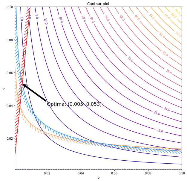
Thus, the smallest value of the contour that touches the feasible region defines the solution for the design problem which is,
$$
\begin{aligned}
b &= 0.005 m\\
d &= 0.053 m\\
W &= 1.98 kg
\end{aligned}
$$