Introduction
The human hip bone is a complex bone structure that functions as the major supporting structure for weight as well as effective transmission of load between the upper and lower body. It has spongy trabecular bones sandwiched in a thin corticular bone shell. Prior works on topology optimization of hip bone have been either limited by solid design resulting in heavy structure or by homogeneity of lattice cells which are not allowed to vary spatially. This work presents the multi-scale optimization of the human hip bone’s topology and microstructure considering the mechanical loads developed during the gait cycle. This may lead to lightweight stiff construction that fits the functional needs of the hip bone.
Problem Statement
The method implemented by Agrawal and Ananthasuresh (2021) has been adopted for the implementation of the lattice structure in the human hip bone. The objective is
to minimize the compliance of the hip bone structure with a weighted multi-load approach for different stages of walking with constraints on mass and porosity helping it mimic the natural properties of the hip bone.
to obtain a design parameterization and technique to incorporate the heterogeneity of lattice structure in the human hip bone.
Methodology
The methodology mainly consists of three steps: Mesh Generation, Boundary conditions and the Optimization algorithm.
Mesh Generation
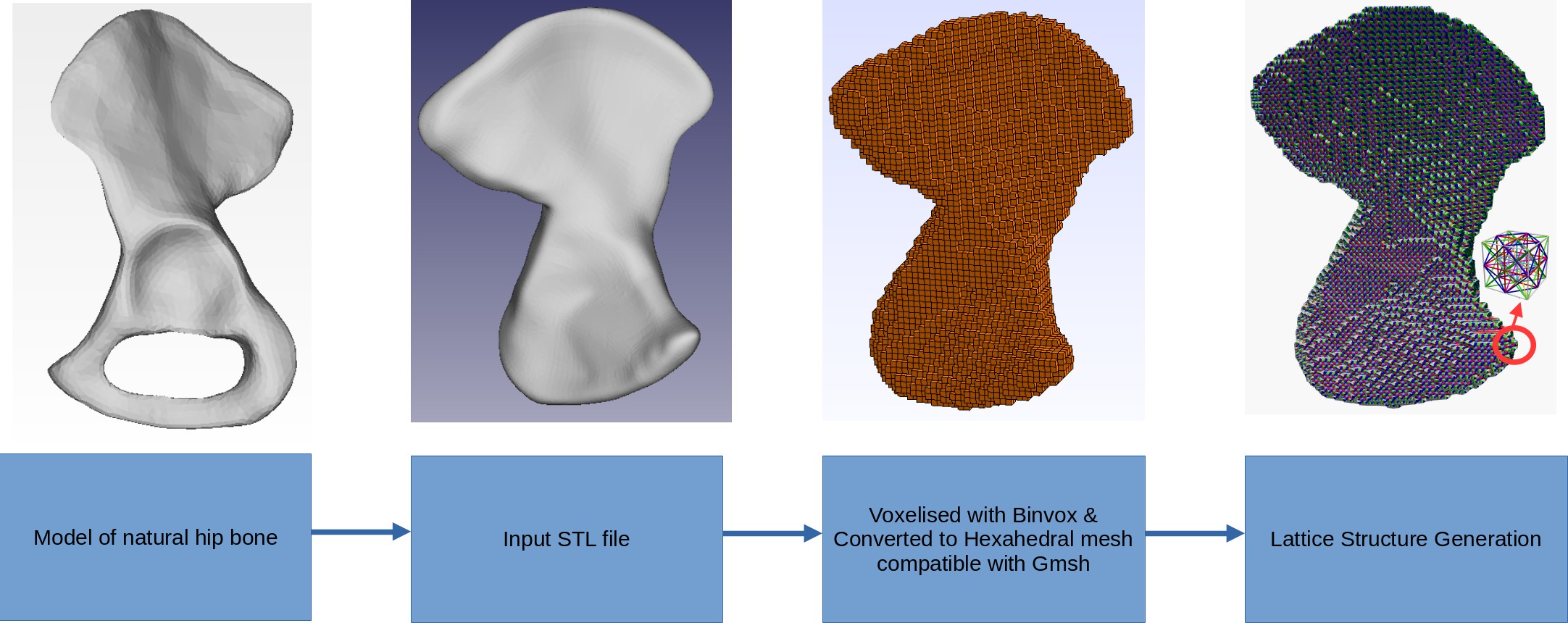 The input design domain for the topology optimization is not made arbitrary due to the boundary conditions imposed by the muscle attachment areas. Hence the model of natural hip bone is converted into a highly constrained input with the obturator foramen hole filled up. This is voxelised and then lattice mesh is generated.
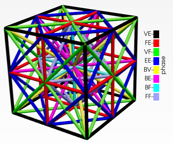
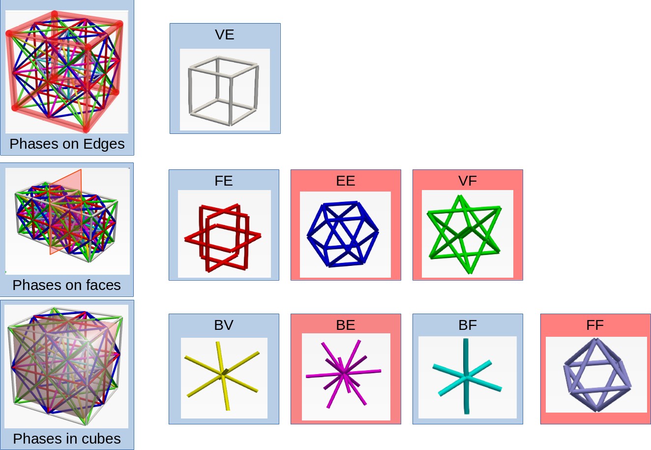
The lattice structure has eight distinct phases that are permitted to occupy a single unit cell. None of the beam elements are collinear but they may intersect. These intersections are generated as separate nodes. A density parameter ($\rho$) is assigned to each phase and its cross-sectional area is proportionate to the density. A phase is absent if density is below minimum limit. Thus $2^8$ distinct phase combinations are available (including the absence of all phases). This unit cell is represented in figure below. The lattice structure is generated by taking the unique combinations of elements connecting eight vertices V, twelve edge centers E, six face centers F and one body center B as shown below. The materials for the beam elements are assumed to be that of cortical bone. It has Young’s modulus of 17000 MPa, poisson’s ratio of 0.3 and density of 1900 kg/$m^{-3}$.
The input design domain for the topology optimization is not made arbitrary due to the boundary conditions imposed by the muscle attachment areas. Hence the model of natural hip bone is converted into a highly constrained input with the obturator foramen hole filled up. This is voxelised and then lattice mesh is generated.
The lattice structure has eight distinct phases that are permitted to occupy a single unit cell. None of the beam elements are collinear but they may intersect. These intersections are generated as separate nodes. A density parameter ($\rho$) is assigned to each phase and its cross-sectional area is proportionate to the density. A phase is absent if density is below minimum limit. Thus $2^8$ distinct phase combinations are available (including the absence of all phases). This unit cell is represented in figure below. The lattice structure is generated by taking the unique combinations of elements connecting eight vertices V, twelve edge centers E, six face centers F and one body center B as shown below. The materials for the beam elements are assumed to be that of cortical bone. It has Young’s modulus of 17000 MPa, poisson’s ratio of 0.3 and density of 1900 kg/$m^{-3}$.
 |
|---|
| A lattice unit cell |
 |
|---|
| Phases in the lattice structure |
Design Parameterization
Each of the phase in an unit cell is associated with a density parameter. This can be represented in an array form as,
where $m$ is the number of phases in each cell and $n$ is the number of cells in the mesh. When the density value is one, the diameter is given by $d=l/3$. Some of these beam elements might be shared between phases. Hence, a redundancy index $n_k$ is defined. The cross-section area is,
where $\mathrm{S_k}$ is the set of all cells that share the $k^{th}$ element.
Boundary Conditions
 | 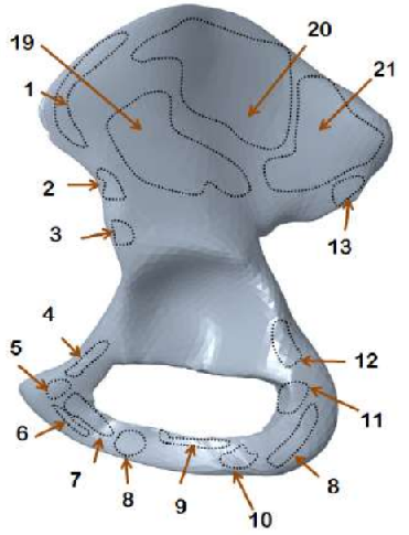 | 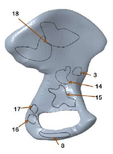 | 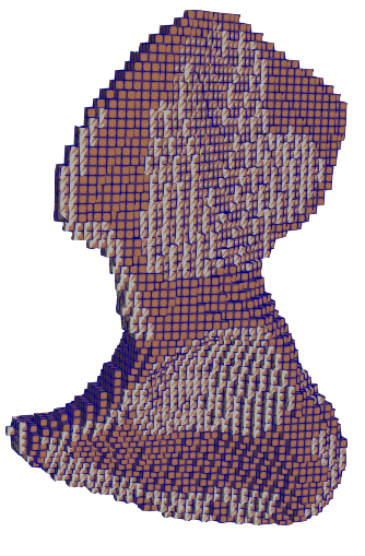 |
|---|---|---|---|
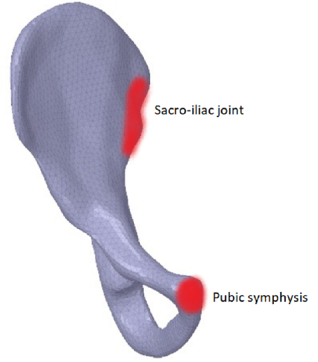
| Dirichlet boundaries | Exterior muscle attachment areas | Interior muscle attachment areas | Boundaries in voxelised domain |
The hip bone is rigidly fixed at pubis-symphysis and sacro-iliac joints. Loads are applied at the acetabulum (hip joint) and twenty one muscle attachment areas as show above. The multi-load approach uses a weighted combination of eight different load conditions. The force conditions modelled in Dalstra and Huiskes (1995) are used for this work. The gait cycle is divided into eight stages. In each stage, the hip joint and muscle forces are applied as static loads.
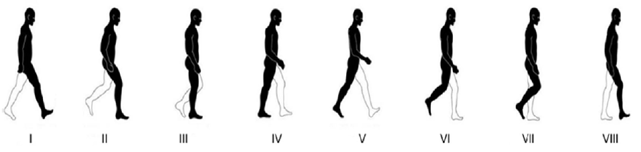 |
|---|
| Eight stages of walking |
Optimization Formulation
The topology optimization problem for the gait cycle can be defined as the minimization of the weighted mean compliance as seen below:
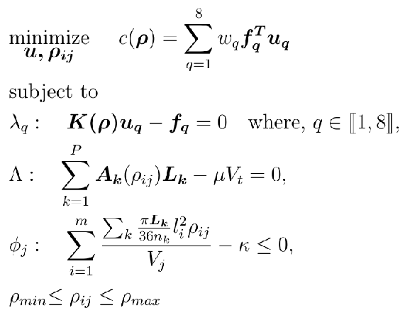
Here $\bm u_q$ and $\bm f_q$ are the global displacement and force vectors respectively for the $q_{\text{th}}$ stage of the gait cycle. $\bm{K(\rho)}$ is the global stiffness matrix. $\lambda_q$, $\Lambda$, $\phi_j$ are the Lagrangian multipliers for the governing equation, volume constraint and porosity constraint respectively. $\mathbf{L_k}$ is the length of the beam segment, $\mu$ is the volume ratio and $V_t$ is the total volume of the design domain. The total volume of beam segments in a cube should be less than $\kappa$ times the volume $V_j$ of the unit cell’s cubic domain.
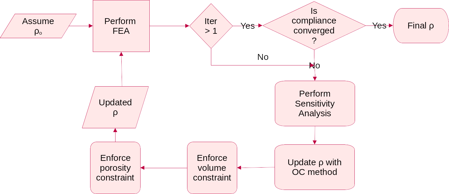
Optimality Criteria Method
The optimization problem defined in above section could be solved using OC method. The update of the density variable is defined as follows:
 |
|---|
| Numerical Algorithm for the Optimality Criteria update |
Results
The project is implemented using Julia programming language and cross-validated with Agrawal and Ananthasuresh (2021) for a case of simple cantilever beam. Two different cases of volume constraints are considered. Case 1: Total mass of the hip bone and Case 2: Mass of the trabecular region of the hip bone. These are converted into equivalent target volumes. The porosity constraint is chosen to be 40% of the unit cell so that Timoshenko beam assumption stays valid. The optimality criteria algorithm was executed with $\beta = 0.5$ subjected to the aforementioned constraint parameters. The following table lists the results corresponding to two cases.
|  | |||||||||||||||||||||
|---|---|---|---|---|---|---|---|---|---|---|---|---|---|---|---|---|---|---|---|---|---|---|
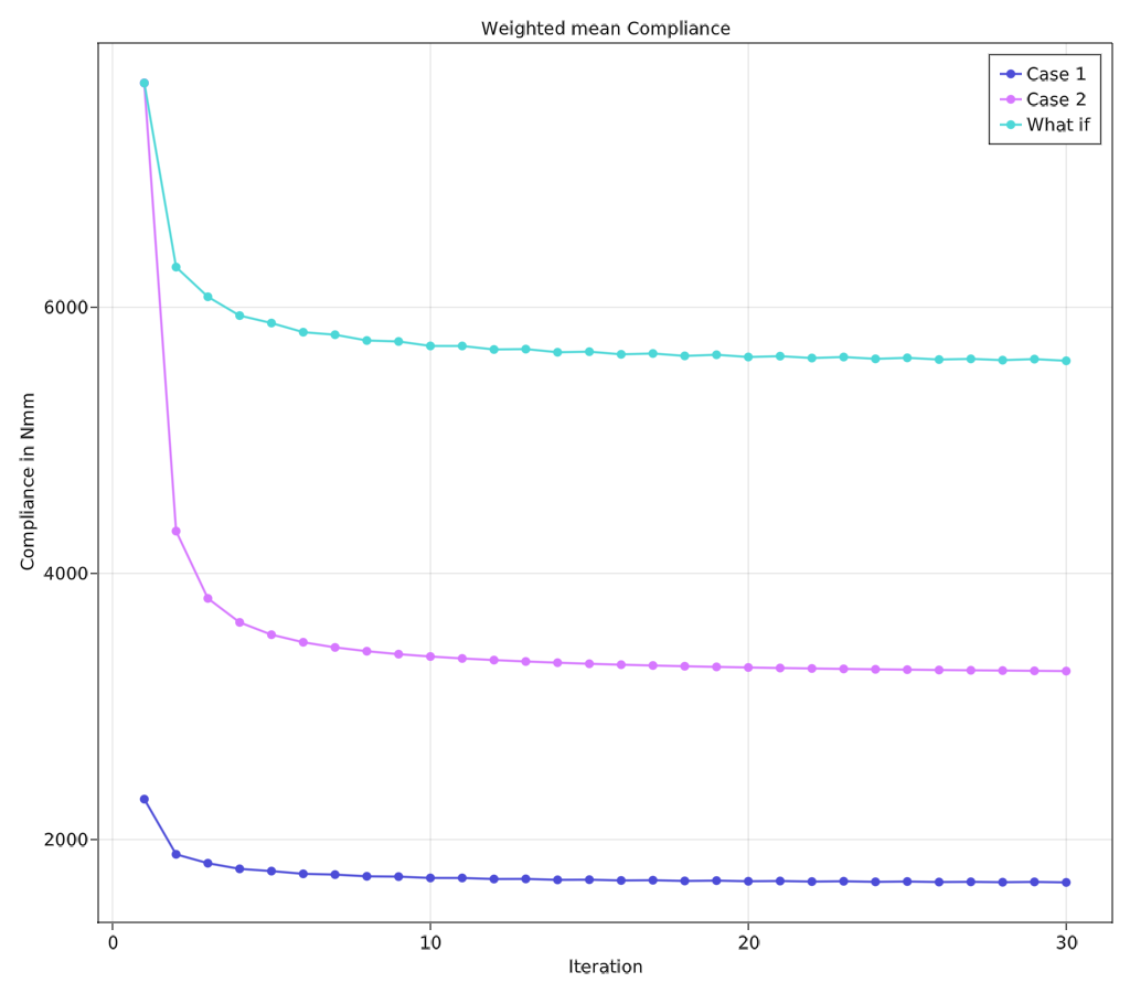
| Compliance values after convergence | Comparison of the compliances |
The above figure shows that case 2 achieves a total reduction of 57.5% of compliance compared to 27.2% in case 1. This shows that this algorithm is very good at creating stiffer structures at lower volume ratios. This could also be associated with the difference between the maximum porosity limit and volume limit. This comparison is listed in table on the left. The figure’s third category “what if” shows how case 1 would compare to case 2 if they had the same initial compliance values.
Output Mesh
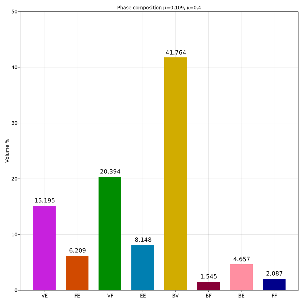
Both cases generate similar mesh with almost same phase composition (percentage volume of each phase compared to total volume). Case 2 had more prominent distinction of phases as various sections of case 2 are scaled up and shown in figure below.
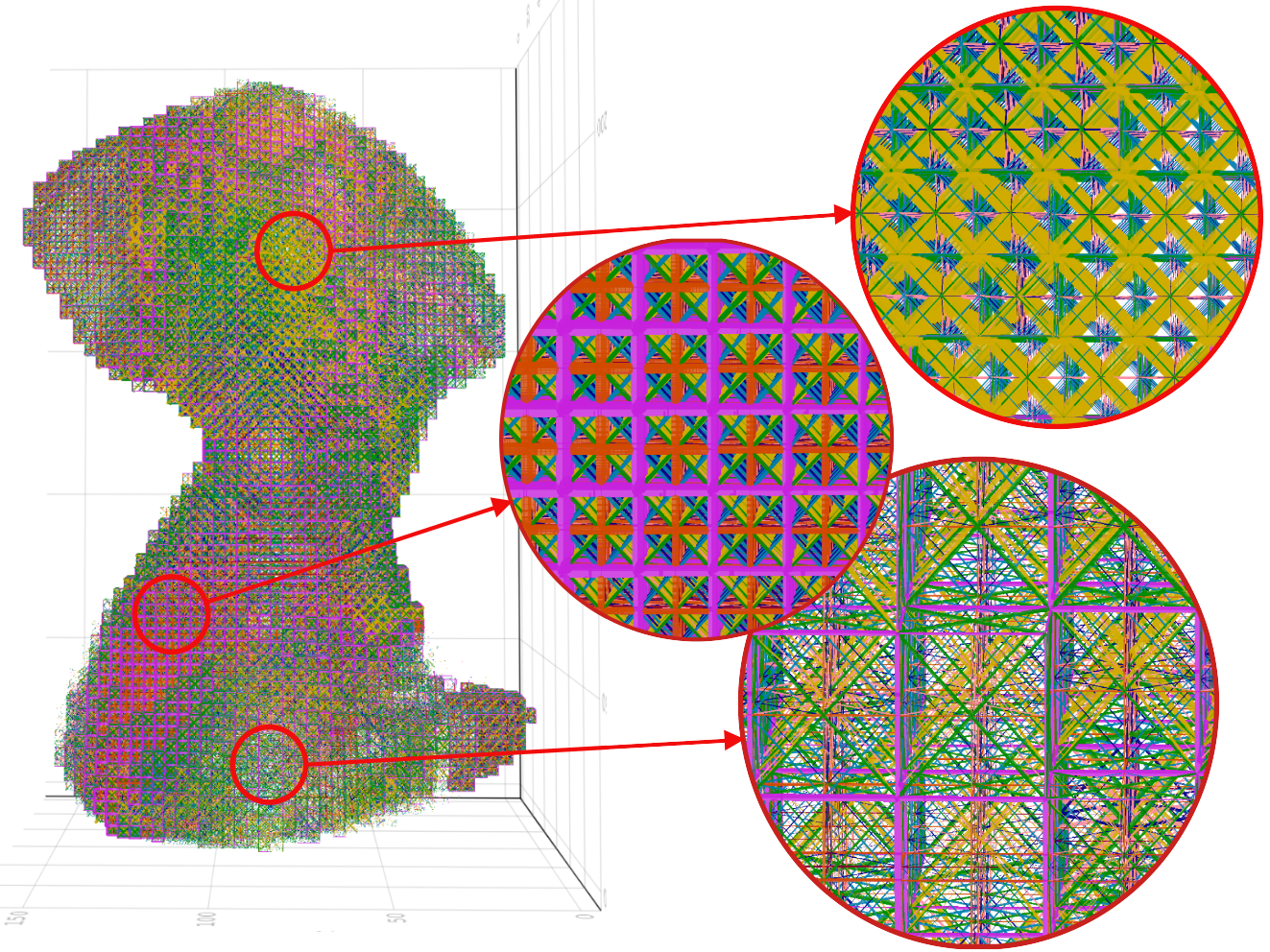
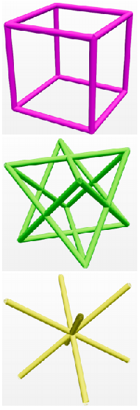
It can be observed that the areas where the obturator foramen occurs in the natural hip bone correspond to very thin beam elements in the case of output mesh as compared to other regions. The thicker regions of the hip bone such as attachment areas of gemellus muscles are predominant with VE phases (pink in colour). The thinner regions of the hip bone such as the attachment areas of gluteus muscles are predominantly covered with BV phases (yellow in colour). The top three dominant phases are BV, VF and VE ranked in that order.
 |  |
|---|---|
| Phase composition for case 2 | VE, VF and BV phases |
It can be observed that the heterogeneity of the lattice structure throughout the design domain has been successfully implemented as detailed in output mesh. One of the surprising results has been the predominance of the BV phase, an octahedral structure, in the phase composition shown in bar plot. Hip bone is mainly a bending dominant structure and hence cubic lattice (VE phase) was expected to be the optimal phase as seen in Agrawal and Ananthasuresh (2021). However, this deviation can be attributed to the size effect of the lattice structure. Yang, 2015 showed that octahedral lattice becomes stiffer as the number of layers decreases. Since hip bone is a tabular and primarily thin structure, the BV phase becomes a more suitable candidate. The next highest-ranked phase is VF which is a predominant phase for structures undergoing torsion or shear. This matches the expectations as the offset in the fixed joints and the hip joint generates a considerable amount of torsion on the structure.
Further, it has been observed that this method results in a very high reduction in the compliance for the case of optimising for the trabecular region of the hip bone. This shows the capability of the method to create an optimal and stiff replacement for the trabecular region of the hip bone.
Future Work
One of the major shortcomings of the current implementations has been the coarseness of the mesh. This limitation has arisen due to the exponential growth in memory requirements for computation. Doubling the grid size from 64 to 128 results in a global stiffness matrix of size around 13 million. Solving this in a single node is impossible with Cholesky (current method of solving) in limited memory and will need iterative solvers which make use of distributed clusters.
The current compliance values achieved are still higher than those achieved in homogenization-based methods Rajaraman and Rakshit (2021). However, this is acceptable since the cortical shell will be simulated in those cases which is not possible in our case. Also, Dalstra and Huiskes, (1995) showed that stresses induced in the cortical shell are nearly 50 times higher than those in the trabecular region. Hence, the current results combined with shell-based implementation of cortical shells may result in a stiff and lightweight structure with the added advantage of heterogeneity over homogenization-based methods.