Generate Logistic Map in Fortran

I had been following the MOOC “Scientific Computing with Fortran” for a week and currently doing the exercises. This is one of the assignments which has piqued my interests - Logistic map. Here’s a neat animation from Wikimedia for the same.

Logistic map animation

As Wikipedia states it, “The logistic map is a polynomial mapping (equivalently, recurrence relation) of degree 2, often cited as an archetypal example of how complex, chaotic behaviour can arise from very simple non-linear dynamical equations”. It is given by the equation, $$ x_{n+1} = rx_n(1-x_n) $$ where,

$x_n \in (0, 1)$
$r \in [-2,4]$ (just to keep the final $x_n$ values bound to $[-0.5, 1.5]$)

I have written the following Fortran code (along with a simple GnuPlot script) to generate the plot.

 1
 2
 3
 4
 5
 6
 7
 8
 9
10
11
12
13
14
15
16
17
18
19
20
21
22
23
24
25
26
27
28
29
30
31
32
33
34
35
36
37
38
39
40
41
42
43
44
45
46
47
48
49
50
51
52
53
54
55
56
57
58
59
60
61
62
63
64
65
66
67
program logisticmap2
    use, intrinsic :: iso_fortran_env, only : error_unit, dp=>real64
    ! i, j, k are integers used for indexing
    implicit integer(i-k)
    ! n is the number of iterations
    ! r_n is the number of elements in r (ranging from r0 to 4)
    ! x0_n is the number of elements in initial x value, ranging from 0 to 0.99
    integer, parameter :: n=3, r_n=1001, x0_n = 101
    real(dp) :: r_vals(r_n), x0_vals(x0_n), xn, r0
    ! xn_vals is a (r_n x x0_n) matrix for final output
    real(dp) :: xn_vals(r_n, x0_n)
    ! Parameters for IO
    integer :: istat, fn
    character(len=1024) :: msg

    ! Getting the initial r value from user 
    print *, "Enter initial r0 value: "
    read(*,*) r0

    ! Generate r and x0 values
    r_vals=linspace(r0, 4._dp, r_n)
    x0_vals=linspace(0.0_dp, 0.99_dp, x0_n)
    
    ! Generate and fill data
    do i = 1,x0_n
        xn = x0_vals(i)
        do j = 1, r_n
            do k= 1, n
                xn = r_vals(j)*xn*(1-xn)
            end do
            xn_vals(j, i) = xn
        end do
    end do

    ! Write to txt file
    open(newunit=fn, file='logisticmap2.txt', access='sequential', &
         status='old', action='write', form='formatted', iostat=istat, iomsg=msg)
    ! Simpler command is as follows:
    ! open(newunit=fn, file='logisticmap2.txt')
    do i=1, r_n
        write(fn, *) r_vals(i), xn_vals(i,:)
        if (istat /= 0) then
            ! Error handling, in case
            write(error_unit, *) msg
            close(fn)
            stop 1
        end if
    end do
    close(fn)
    ! calling the gnuplot to plot logisticmap2.plt file
    call execute_command_line('gnuplot -p logisticmap2.plt')

    
    contains
    ! A linspace function similar to matlab
    function linspace(x0, xn, n) result(x)
        integer, intent(in):: n
        integer :: i
        real(dp), intent(in):: x0, xn
        real(dp) :: x(n)
        real :: step
        step=(xn-x0)/(n-1)
        do i=1,n
            x(i) = x0 + step*(i-1)
        end do
    end function linspace
end program logisticmap2

And the following is store in the logisticmap2.plt file.

1
2
3
4
5
6
7
set nokey
set grid
set title "Logistic Map X_{n+1}=r X_n(1-X_n) with (n=3)"
set xlabel "r"
set ylabel "X_n"
m="logisticmap2.txt"
plot for [col=2:101] m using 1:col with d

I have generated the plot for various initial r values,which pertains to different zoom levels.

logisticmap1

logisticmap3

logisticmap3_5

logisticmap3_84

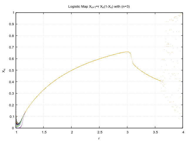
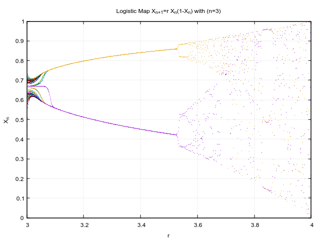
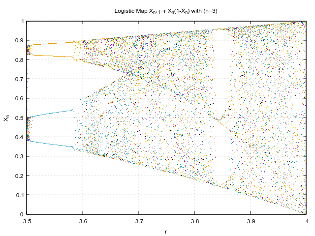
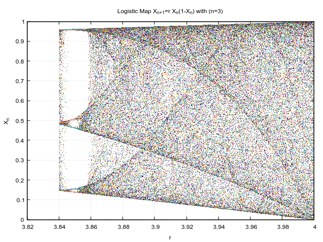
I like how such chaotic behaviour rises out of seemingly simple equation and that too in just 3 iterations! Just to put in perspective, this is how the initial conditions looked like.

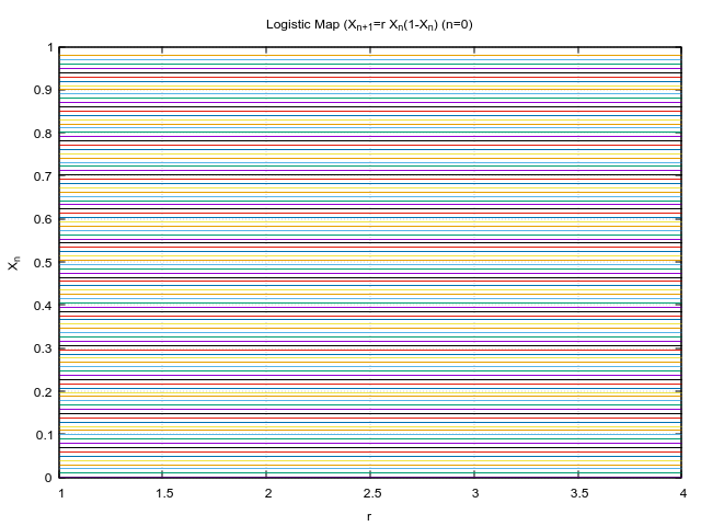
logisticmapn0

Generate Logistic Map in Fortran

See Also: