Linearization of Single Variable Non-Linear function

Linearization is a way to approximate a non-linear function around a point. In the blog post, I’ll show an implementation of best linearization of an equation around a point using Newton-raphson method. Before proceeding further, please note the following.

1. Newton raphson is better suited for monotonic functions or in the regions where monotonic behaviour is seen. Hence, my implementation is not ideal condition.
2. Newton Raphson may not converge if the equation may achieve a horizontal or vertical slope before the required point.

Now, with that out of the way, let me show you cool function which I tried to linearize.

Problem Statement

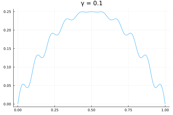
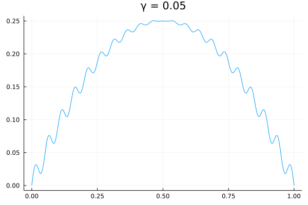
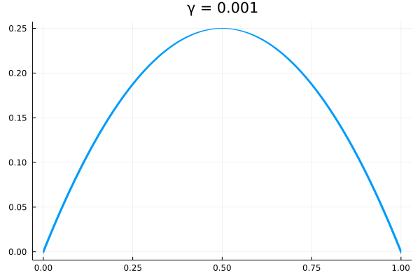
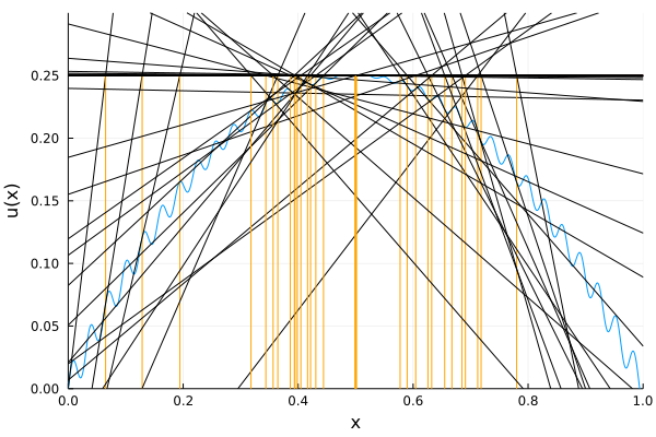
Consider the following non-linear equation. $$ \displaystyle{u\left( x \right) = x - x^2 + \sqrt\gamma\left( \frac{1}{4\pi}\sin\left( \frac{2\pi x}{\gamma} \right)- \frac{x}{2\pi}\sin\left( \frac{2\pi x}{\gamma} \right) -\frac{\gamma}{4\pi^2}\cos\left( \frac{2\pi x}{\gamma} \right) + \frac{\gamma}{4\pi^2} \right) } $$ where $x \in [0,1]$ and $\gamma$ is a parameter that ranges from $10^{-1}$ to $10^{-2}$. The resulting plots for this equation for various set of $\gamma$ values are as follows:

Derivation of linear equation

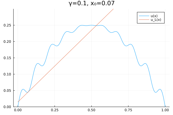
The linearized equation is of the form, $$ \displaystyle{u_L(x) = c_1 + c_2 x} $$ Applying the boundary conditions at index $i=0$,

we get,

$$ \displaystyle{u_L(x) = u(x_0) + u’(x_0)(x-x_0)} $$

where,

$$ \displaystyle{u’(x) = (1-2x) \left( 1+ \frac{1}{2\sqrt{\gamma}}\cos\left(\frac{2\pi x}{\gamma} \right) \right) } $$

Algorithm

Rearranging $u_L(x)$ in terms of $x$ and substituting $u_L(x) = u(x^*)$, we get $$ x_{i+1} = x_i + \frac{u(x^*) - u(x_i)}{u’(x_i)} $$ Then, the code is generated as per following pseudocode.

1
2
3
4
5
6
7
8

Ɛ = 1e-11
x_i = 0
x* = 0.5

repeat
	x_i+1 = x_i + (u(x*) - u(x_i))/u'(x_i)
	residue = |u(x*) - u_l(x*)|
while residue > Ɛ

Convergence

Solution 1

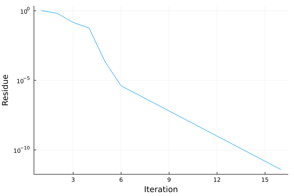
Here’s the Convergence of solution with $x_0=0.0, \gamma=0.1$

This was done in 17 iterations.

Solution 2

Here is another solution which took quite a detour before convergence. This is the convergence of solution with $x_0=0.0, \gamma=0.031$ which took 87 iterations.

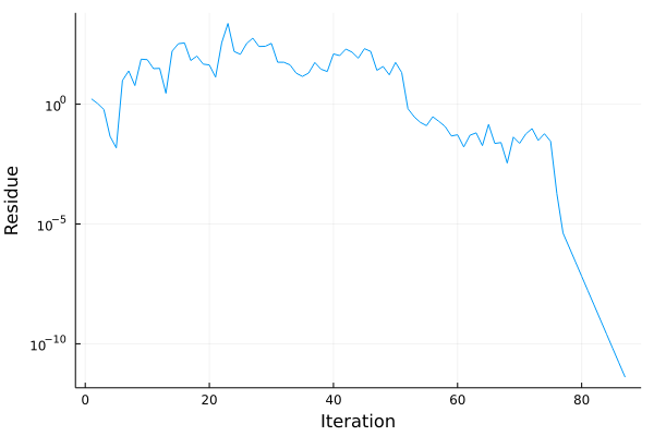
There is no exact way to predict the iterations or whether it will converge because the equation doesn’t satisfy the conditions meant for the newton raphson.

Convergence for various parameter values

To get the general idea of convergence, I generated a surface plot of $\frac 1 {\text{No of iterations}}$ for various initial conditions and parameter values - $x_0\in[0,1], \gamma\in[0.01, 0.1]$.

Here, I had to truncate the height to 0.15 since, for the exact condition $x_0 = x^*$, the equation was linearized in one iteration. The peaks represent lesser iterations than the trough.

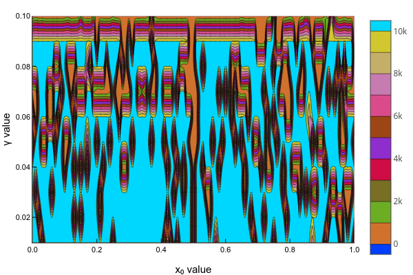
I also generated a contour plot of the number of iterations ranging upto 10,000 iterations which I had set as the maximum limit.

I had generated the above code as a python notebook which can be found here or it can be run directly online using binder if you follow this link.