Visualizing 1D & 2D FEM Basis Functions in Julia

The Finite Element Method (FEM) is a mathematical tool using for solving differential equations. It has been popularly used (also, initially developed) for solving elastostatics problems which is to find the displacement uu such that, σij,j+fi=0 in the domain Ω \sigma_{ij,j} + f_i = 0 \text{ in the domain }\Omega To solve this, the domain Ω\Omega is split into finite sub domains Ωe\Omega_e in which the solution uu is (usually) approximated by a polynomial of certain order which is governed by the regularity requirements of the weak form of above PDE.

The division into finite elements Ωe\Omega_e is usually done as

  • Lines for 1D problem (obviously)
  • Quadrilaterals in 2D problems
  • Hexahedrons in 3D problems

These finite elements are then mapped to a “Natural co-ordinate” system where they accordingly become

  • Lines with ξ1(1,1)\xi_1 \in (-1,1)
  • Square with ξ1,ξ2(1,1)\xi_1, \xi_2 \in (-1,1)
  • Cubes with ξ1,ξ2,ξ3(1,1)\xi_1, \xi_2, \xi_3 \in (-1,1)

where ξ1,ξ2,ξ3\xi_1, \xi_2, \xi_3 are the x,y,zx,y,z co-ordinates in this bi-unit domain (called so since these values here range from 1-1 to 11).

While the FEM is solved for discrete values of uu, the solution is presented as a continuous function over the domain as well as within the elements. This equation of the solution is obtained by scaling the Lagrangian polynomials in this space by the nodal values of uu (it is these nodal values that FEM finally solves for). These Lagrangian polynomials are (usually) the basis functions of the finite elements.
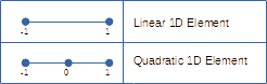
1-D Elements

See

FEM1Delements

The above diagram shows the nodes for 1D elements. There are two main points to be noted:

  • There are polynomials for each node of an element. And these polynomials are chosen such a way that these polynomials have value 11 at that node and 00 at all other nodes.
  • Order of the polynomial =Number of nodes1=\text{Number of nodes}-1

The final solution is the sum of all these polynomials which can be given as u(ξ)=A=1NnodesNA(ξ)uA u(\xi) = \sum_{A=1}^{N_{\text{nodes}}}N_A(\xi)\bf u_A where,

  • NAN_A is the basis function at node A.
  • uA\bf u_A is nodal degree of freedom (value of displacement).
  • NnodesN_\text{nodes} is the total number of nodes per element.

The general Lagrangian basis function NAN_A is given as, NA(ξ)=B=1BANnodesξξBξAξB N_A(\xi) = \prod_{B=1 \\ B\not=A}^{N_\text{nodes}}\frac {\xi - \xi_B}{\xi_A - \xi_B} where BB iterates through all the nodes except A. It can be observed here that the value of basis function is always zero at all the nodes (except A).

 1
 2
 3
 4
 5
 6
 7
 8
 9
10
11
12
# The generic Lagrangian basis function is
function N(ξ, order, node)
	ξ_B = range(-1, 1, length=order+1) |> collect
	ξ_A = ξ_B[node]
	N_A = 1
	for i in range(1, order+1)
		if i  node
			N_A *= (ξ - ξ_B[i])/(ξ_A - ξ_B[i])
		end
	end
	N_A
end

Note that, we won’t be using the generic function for the ease of comparison of various orders. Now that we are moving into plotting of basis functions, let me initialize the prerequisites in Julia.

1
2
3
4
using Plots
plotly()

ξ₁ = ξ₂ = range(-1, 1, step=0.01) |> collect

1D Linear Element

For linear elements, substituting the nodal ξ\xi values in the above basis function, we get the shape functions as follows,

N11(ξ)=1ξ2N21(ξ)=1+ξ2 N_1^1(\xi) = \frac {1-\xi}{2} \\ N_2^1(\xi) = \frac {1+\xi}{2}

The superscript 1 denotes that it is a linear element. The same basis functions can be obtained by calling the above function as N(ξ, 1, node) for each of the respective node. The corresponding plots are,

1
2
3
4
5
6
7
8
N₁1(ξ) = (1-ξ)/2
N₂1(ξ) = (1+ξ)/2
plt1 = plot(N₁1, -1, 1, title="N₁")
plt2 = plot(N₂1, -1, 1, title = "N₂")
plot(plt1, plt2, 
	legend=false,
	xlabel="ξ₁",
	ylabel="N")
−1.0−0.50.00.51.00.000.250.500.751.00−1.0−0.50.00.51.00.000.250.500.751.00
N₁N₂

1D Quadratic Element

The quadratic shape function is given as,

N12(ξ)=ξ2ξ2N22(ξ)=ξ22N22(ξ)=ξ2+ξ2 \begin{aligned} N_1^2(\xi) &= \frac {\xi^2-\xi}{2} \\ N_2^2(\xi) &= \frac {\xi^2}{2} \\ N_2^2(\xi) &= \frac {\xi^2+\xi}{2} \end{aligned}
Again, the superscript 22 denotes that its order is 2.
 1
 2
 3
 4
 5
 6
 7
 8
 9
10
N₁2(ξ) = (ξ-1)ξ/2
N₂2(ξ) = 1-ξ^2
N₃2(ξ)	= (ξ+1)ξ/2
plt1 = plot(N₁2, ξ₁, title="N₁")
plt2 = plot(N₂2, ξ₁, title = "N₂")
plt3 = plot(N₃2, ξ₁, title = "N₃")
plot(plt1, plt2, plt3,
	legend=false,
	xlabel="ξ₁",
	ylabel="N")
−1.0−0.50.00.51.00.000.250.500.751.00−1.0−0.50.00.51.00.000.250.500.751.00−1.0−0.50.00.51.00.000.250.500.751.00
ξ₁ξ₁ξ₁NNNN₁N₂N₃

1D Cubic Element

The cubic shape function is,

N13(ξ)=116(9ξ39ξ2ξ+1)N23(ξ)=116(27ξ39ξ227ξ+9)N23(ξ)=116(27ξ3+9ξ227ξ9)N43(ξ)=116(9ξ3+9ξ2ξ1) \begin{aligned} N_1^3(\xi) &= \frac{-1}{16}(9\xi^3 - 9\xi^2 - \xi + 1) \\ N_2^3(\xi) &= \frac{1}{16}(27\xi^3 -9\xi^2 -27\xi + 9) \\ N_2^3(\xi) &= \frac{-1}{16}(27\xi^3 + 9\xi^2 - 27\xi - 9) \\ N_4^3(\xi) &= \frac{1}{16}(9\xi^3 + 9\xi^2 - \xi - 1) \end{aligned}
 1
 2
 3
 4
 5
 6
 7
 8
 9
10
11
12
N₁3(ξ) = -(9ξ^3 - 9ξ^2 - ξ + 1)/16
N₂3(ξ) = (27ξ^3 -9ξ^2 -27ξ + 9)/16
N₃3(ξ) = -(27ξ^3 + 9ξ^2 -27ξ - 9)/16
N₄3(ξ)	= (9ξ^3 + 9ξ^2 - ξ - 1)/16
plt1 = plot(N₁3, ξ₁, title="N₁")
plt2 = plot(N₂3, ξ₁, title = "N₂")
plt3 = plot(N₃3, ξ₁, title = "N₃")
plt4 = plot(N₄3, ξ₁, title = "N₄")
plot(plt1, plt2, plt3, plt4,
	legend=false,
	xlabel="ξ₁",
	ylabel="N")
−1.0−0.50.00.51.00.000.250.500.751.00−1.0−0.50.00.51.0−0.20.00.20.40.60.81.0−1.0−0.50.00.51.0−0.20.00.20.40.60.81.0−1.0−0.50.00.51.00.000.250.500.751.00
ξ₁ξ₁ξ₁ξ₁NNNNN₁N₂N₃N₄

2D Elements

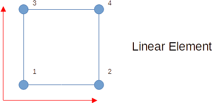
For the case of 2D elements, we will consider the quadratic elements which can be obtained as a tensor product of the above 1D basis functions. This can be represented as,

N=Nξ1Nξ2Nij=NiNj \begin{aligned} \bf N &= N^{\xi_1} \otimes N^{\xi_2}\\ \bf N_{ij} &= N_i N_j \end{aligned}
Generally, an element has the same order of the basis functions along both ξ1\xi_1 and ξ2\xi_2 directions though it need not be the case.

Thus, for a quadilateral element, the basis function in the natural co-ordinates (where it is transformed to square elements) over each node can be obtained by tensor product as,

N=[N1N2Nn][N1N2Nn]=[N1N1N1N2N1NnN2N1N2N2N2NnNnN1NnN2NnNn] \begin{aligned} \mathbf{N} &=\left[\begin{array}{c} N_{1} \\ N_{2} \\ \vdots \\ N_{n} \end{array}\right] \otimes \left[\begin{array}{c} N_{1} \\ N_{2} \\ \vdots \\ N_{n} \end{array}\right] \\ &= \left[\begin{array}{cccc} N_{1} N_{1} & N_{1} N_{2} & \cdots & N_{1} N_{n} \\ N_{2} N_{1} & N_{2} N_{2} & \cdots & N_{2} N_{n} \\ \vdots & \vdots & \ddots & \vdots \\ N_{n} N_{1} & N_{n} N_{2} & \cdots & N_{n} N_{n} \end{array}\right] \end{aligned}

2D Linear Elements

2D Linear Elements

For the linear elements, following the previous notations we can obtain the shape function as,

N=[N1N2][N1N2]=[N1N1N1N2N2N1N2N2] \bf{N} =\left[\begin{array}{c} N_{1} \\ N_{2} \end{array}\right] \otimes \left[\begin{array}{c} N_{1} \\ N_{2} \\ \end{array}\right] = \left[\begin{array}{cc} N_{1} N_{1} & N_{1} N_{2} \\ N_{2} N_{1} & N_{2} N_{2} \end{array}\right]
In the same spirits, the julia code can be created as the outer outer of the 1D linear element vector as
1
2
N1(ξ) = [N₁1(ξ), N₂1(ξ)]
N2(ξ1, ξ2) = N1(ξ1)*N1(ξ2)'

But, for the readability, we will follow the elementwise multiplication as instead of the above seen code.

1
2
3
4
5
6
7
8
9
N₁₁1(ξ1, ξ2) = N₁1(ξ1)*N₁1(ξ2)
N₁₂1(ξ1, ξ2) = N₁1(ξ1)*N₂1(ξ2)
N₂₁1(ξ1, ξ2) = N₂1(ξ1)*N₁1(ξ2)
N₂₂1(ξ1, ξ2) = N₂1(ξ1)*N₂1(ξ2)
s11=surface(ξ₁, ξ₂, N₁₁1, title="N₁₁")
s21=surface(ξ₁, ξ₂, N₁₂1, title="N₁₂")
s31=surface(ξ₁, ξ₂, N₂₁1, title="N₂₁")
s41=surface(ξ₁, ξ₂, N₂₂1, title="N₂₂")
plot(s11,s21,s31,s41)

Here is the plot for the N11N_{11}. The zz axis represents the nodal values of the shape function while the xyxy plane represents the vector field of ξ1\xi_1 and ξ2 \xi_2.

One interesting point to observe here is that, though the function is linear, the plot is curved along the diagonal. That is because the shape function is actually a bilinear function of ξ1\xi_1 and ξ2\xi_2. Here is the plot for each shape functions.

00.20.40.60.8100.20.40.60.8100.20.40.60.8100.20.40.60.81N₁₁N₁₂N₂₁N₂₂

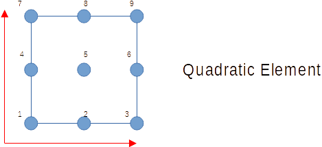
2D Quadratic Elements

2D Linear Elements

The quadratic elements are obtained through the tensor product as,

N=[N1N2N3][N1N2N3]=[N1N1N1N2N1N3N2N1N2N2N2N3N3N1N3N2N3N3] \bf{N} =\left[\begin{array}{c} N_{1} \\ N_{2} \\ N_{3} \end{array}\right] \otimes \left[\begin{array}{c} N_{1} \\ N_{2} \\ N_{3} \end{array}\right] = \left[\begin{array}{ccc} N_{1} N_{1} & N_{1} N_{2} & N_{1} N_{3}\\ N_{2} N_{1} & N_{2} N_{2} & N_{2} N_{3}\\ N_{3} N_{1} & N_{3} N_{2} & N_{3} N_{3} \end{array}\right]
 1
 2
 3
 4
 5
 6
 7
 8
 9
10
11
12
13
14
15
16
17
18
19
N₁₁2(ξ1, ξ2) = N₁2(ξ1)*N₁2(ξ2)
N₁₂2(ξ1, ξ2) = N₁2(ξ1)*N₂2(ξ2)
N₁₃2(ξ1, ξ2) = N₁2(ξ1)*N₃2(ξ2)
N₂₁2(ξ1, ξ2) = N₂2(ξ1)*N₁2(ξ2)
N₂₂2(ξ1, ξ2) = N₂2(ξ1)*N₂2(ξ2)
N₂₃2(ξ1, ξ2) = N₂2(ξ1)*N₃2(ξ2)
N₃₁2(ξ1, ξ2) = N₃2(ξ1)*N₁2(ξ2)
N₃₂2(ξ1, ξ2) = N₃2(ξ1)*N₂2(ξ2)
N₃₃2(ξ1, ξ2) = N₃2(ξ1)*N₃2(ξ2)
s12=surface(ξ₁, ξ₂, N₁₁2, title="N₁₁")
s22=surface(ξ₁, ξ₂, N₁₂2, title="N₁₂")
s32=surface(ξ₁, ξ₂, N₁₃2, title="N₁₃")
s42=surface(ξ₁, ξ₂, N₂₁2, title="N₂₁")
s52=surface(ξ₁, ξ₂, N₂₂2, title="N₂₂")
s62=surface(ξ₁, ξ₂, N₂₃2, title="N₂₃")
s72=surface(ξ₁, ξ₂, N₃₁2, title="N₃₁")
s82=surface(ξ₁, ξ₂, N₃₂2, title="N₃₂")
s92=surface(ξ₁, ξ₂, N₃₃2, title="N₃₃")
plot(s12,s22, s32, s42, s52, s62, s72, s82, s92)
N₁₁N₁₂N₁₃N₂₁N₂₂N₂₃N₃₁N₃₂N₃₃

2D Cubic Elements

2D Linear Elements

 1
 2
 3
 4
 5
 6
 7
 8
 9
10
11
12
13
14
15
16
17
18
19
20
21
22
23
24
25
26
27
28
29
30
31
32
33
N₁₁3(ξ1, ξ2) = N₁3(ξ1)*N₁3(ξ2)
N₁₂3(ξ1, ξ2) = N₁3(ξ1)*N₂3(ξ2)
N₁₃3(ξ1, ξ2) = N₁3(ξ1)*N₃3(ξ2)
N₁₄3(ξ1, ξ2) = N₁3(ξ1)*N₄3(ξ2)
N₂₁3(ξ1, ξ2) = N₂3(ξ1)*N₁3(ξ2)
N₂₂3(ξ1, ξ2) = N₂3(ξ1)*N₂3(ξ2)
N₂₃3(ξ1, ξ2) = N₂3(ξ1)*N₃3(ξ2)
N₂₄3(ξ1, ξ2) = N₂3(ξ1)*N₄3(ξ2)
N₃₁3(ξ1, ξ2) = N₃3(ξ1)*N₁3(ξ2)
N₃₂3(ξ1, ξ2) = N₃3(ξ1)*N₂3(ξ2)
N₃₃3(ξ1, ξ2) = N₃3(ξ1)*N₃3(ξ2)
N₃₄3(ξ1, ξ2) = N₃3(ξ1)*N₄3(ξ2)
N₄₁3(ξ1, ξ2) = N₄3(ξ1)*N₁3(ξ2)
N₄₂3(ξ1, ξ2) = N₄3(ξ1)*N₂3(ξ2)
N₄₃3(ξ1, ξ2) = N₄3(ξ1)*N₃3(ξ2)
N₄₄3(ξ1, ξ2) = N₄3(ξ1)*N₄3(ξ2)
s013=surface(ξ₁, ξ₂, N₁₁3, title="N₁₁")
s023=surface(ξ₁, ξ₂, N₁₂3, title="N₁₂")
s033=surface(ξ₁, ξ₂, N₁₃3, title="N₁₃")
s043=surface(ξ₁, ξ₂, N₁₄3, title="N₁₄")
s053=surface(ξ₁, ξ₂, N₂₁3, title="N₂₁")
s063=surface(ξ₁, ξ₂, N₂₂3, title="N₂₂")
s073=surface(ξ₁, ξ₂, N₂₃3, title="N₂₃")
s083=surface(ξ₁, ξ₂, N₂₄3, title="N₂₄")
s093=surface(ξ₁, ξ₂, N₃₁3, title="N₃₁")
s103=surface(ξ₁, ξ₂, N₃₂3, title="N₃₂")
s113=surface(ξ₁, ξ₂, N₃₃3, title="N₃₃")
s123=surface(ξ₁, ξ₂, N₃₄3, title="N₃₄")
s133=surface(ξ₁, ξ₂, N₄₁3, title="N₄₁")
s143=surface(ξ₁, ξ₂, N₄₂3, title="N₄₂")
s153=surface(ξ₁, ξ₂, N₄₃3, title="N₄₃")
s163=surface(ξ₁, ξ₂, N₄₄3, title="N₄₄")
plot(s133,s143,s153,s163, s093,s103,s113,s123, s053,s063,s073,s083, s013,s023,s033,s043, colorbar=false, size=(600, 800))

Again, the cubic 2D element is the tensor product of the 1D shape functions,

N=[N1N2N3N4][N1N2N3N4]=[N1N1N1N2N1N3N1N4N2N1N2N2N2N3N2N4N3N1N3N2N3N3N3N4N4N1N4N2N4N3N4N4] \bf{N} =\left[\begin{array}{c} N_{1} \\ N_{2} \\ N_{3} \\ N_{4} \end{array}\right] \otimes \left[\begin{array}{c} N_{1} \\ N_{2} \\ N_{3} \\ N_{4} \end{array}\right] = \left[\begin{array}{cccc} N_{1} N_{1} & N_{1} N_{2} & N_{1} N_{3} & N_{1} N_{4}\\ N_{2} N_{1} & N_{2} N_{2} & N_{2} N_{3} & N_{2} N_{4}\\ N_{3} N_{1} & N_{3} N_{2} & N_{3} N_{3} & N_{3} N_{4}\\ N_{4} N_{1} & N_{4} N_{2} & N_{4} N_{3} & N_{4} N_{4}\\ \end{array}\right]
N₄₁N₄₂N₄₃N₄₄N₃₁N₃₂N₃₃N₃₄N₂₁N₂₂N₂₃N₂₄N₁₁N₁₂N₁₃N₁₄

Thus a general representation of the Lagrangian basis functions have been achieved for the 1D and 2D elements. I do wish to implement the same for the 3D elements but I seem to be running out of spaces! (Actually, it is possible and will implement and update with link soon). This had been a very good learning experience for me and am looking forward to dwelving more into this realm soon!

Load Comments?