Solving 2nd Order ODEs in Julia

The second order Linear Differential Equations can be solved using DifferentialEquations.jl package available in Julia repository. Here is an example problem being solved using Julia.

Consider a 4-degree of freedom undamped free vibration system as follows.

4dof-system

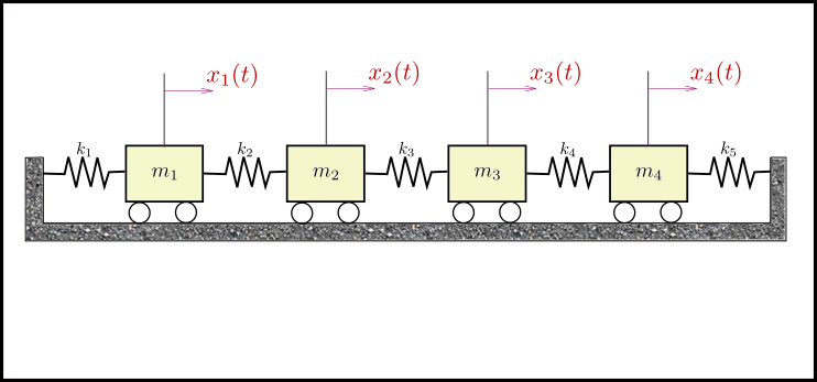
The above system can be represented by the equation,

$\displaystyle{[M] [\ddot{x}] + [K][x] = 0}$

where,

\displaystyle{ \begin{aligned} M &=\begin{bmatrix} m_1 & 0 & 0 & 0 \\ 0 & m_2 & 0 & 0 \\ 0 & 0 & m_3 & 0 \\ 0 & 0 & 0 & m_4 \end{bmatrix} \\ K &=\begin{bmatrix} k_1+k_2 & -k_2 & 0 & 0 \\ -k_2 & k_2+k_3 & -k_3 & 0 \\ 0 & -k_3 & k_3+k_4 & -k_4 \\ 0 & 0 & -k_4 & k_4+k_5 \end{bmatrix} \\ \ddot{x} &=\begin{bmatrix} \ddot x_1 \\ \ddot x_2 \\ \ddot x_3 \\ \ddot x_4 \end{bmatrix}; x =\begin{bmatrix} x_1 \\ x_2 \\ x_3 \\ x_4 \end{bmatrix}\\ \end{aligned} }

Let’s take the following values and initial conditions for this problem.

\displaystyle{ \begin{aligned} M &=\begin{bmatrix} 5 & 0 & 0 & 0 \\ 0 & 5 & 0 & 0 \\ 0 & 0 & 5 & 0 \\ 0 & 0 & 0 & 5 \end{bmatrix} \\ K&=\begin{bmatrix} 10 & -5 & 0 & 0 \\ -5 & 10 & -5 & 0 \\ 0 & -5 & 10 & -5 \\ 0 & 0 & -5 & 5 \end{bmatrix} \\ F &=\begin{bmatrix} 0 \\ 0 \\ 0 \\ 0 \end{bmatrix}; \dot{x}\left( 0 \right) =\begin{bmatrix} 0 \\ 0 \\ 0 \\ 0 \end{bmatrix}; x\left( 0 \right) =\begin{bmatrix} 0.025 \\ 0.02 \\ 0.02 \\ 0.001 \end{bmatrix} \end{aligned} }

1
2
3
4
5
6
7
using DifferentialEquations
M = Array(I(4)*5)
K = Array(Tridiagonal([-5, -5, -5], [10, 10, 10, 5], [-5, -5, -5]))
F = zeros(4)
ẋ₀ = zeros(4)
x₀ = [0.025, 0.02, 0.02, 0.001]
B = -inv(M)*K

The above differential equation can be re-arranged as,

\displaystyle{ \begin{aligned} \ddot{x} &= -[M]^{-1}[K][x] \\ &= [B][x] \end{aligned} }

where, $\displaystyle{[B] = -[M]^{-1}[K]}$ .

Now, to solve the equation $\displaystyle{\ddot{x} = Bx}$ , the following code is run in julia.

1
2
3
4
tspan = (0.0, 200.0)
f(du, u, p, t) = F+B*u
prob = SecondOrderODEProblem(f,ẋ₀,x₀,tspan)
sol = DifferentialEquations.solve(prob)

Some key points to note are,

The solution is arrived as three steps.
1. Define the differential equation f.
2. Define the problem by specifying function, initial conditions and time span.
3. Solving the defined problem.
tspan is the variable which specifies the range over which we are solving for $x$ .
The function f is equated to second derivative $\ddot x$ here. Generally, f is a function of,
1. du - The derivative of u
2. u - The variable being solved
3. p - parameter for parameterized functions
4. t - time
The function SecondOrderODEProblem takes in the function f, initial conditions du0( $\dot x_0$ here) and u0 ( $x_0$ here), and the time span tspan.
solve generates dataset containing 9 columns - timestamp, $\displaystyle{\dot x_1, \dot x_2, \dot x_3, \dot x_4, x_1, x_2, x_3, x_4}$

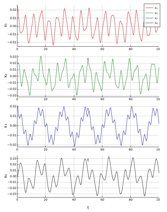
The response (displacement) of the above system can be plotted as follows.

1
2
3
4
5
6
7
8
plot(sol, 
	vars=[5, 6, 7, 8], 
	tspan=(0, 100), 
	layout=(4,1), 
	size=(600, 800),
	ylabel=["x₁" "x₂" "x₃" "x₄"],
	label=["x₁" "x₂" "x₃" "x₄"],
	color=["Red" "Green" "Blue" "Black"])

This is a post I’ve made as part of my learning experience. Let me know if you have any feedback.

Solving 2nd Order ODEs in Julia

See Also: